NGC 2682 is a great example of a cluster with a well-defined main sequence, turn-off point, and red giant population, and in many ways bridges the gap between the young open clusters you analysed in Examples 1–4 and the globular cluster you will analyse in Example 6. Before moving on, it’s worth consolidating the strategies you’ve developed across all the examples so far, since these will serve you well when analysing any cluster — including one you’ve observed yourself.
Process matters. The order in which you approach the analysis is important. Begin by removing field stars, since these obscure the cluster’s true colour-magnitude distribution. Once you have a reasonable estimate of the cluster’s proper motion and distance, fetch archival data out beyond the cluster’s radius to ensure all cluster stars are included, then refine your astrometric constraints. When fitting isochrones, first adjust age and metallicity to match the shape of the turnoff point and red giant branch, and ensure the model runs along the bottom of the main sequence — not through the middle of it. Then adjust distance and reddening to align the model spatially with the data, checking that the fit holds across multiple photometric diagrams simultaneously. Finally, iterate to refine.
Prioritise the bright end. Stars near the top of the HR diagram have more accurate photometric measurements than those near the bottom, where signal-to-noise is lower and scatter is greater. Focus your fitting efforts on the turnoff point, the red giant branch, and the upper main sequence. Don’t sacrifice a good fit to the bright stars for the sake of better matching the scattered faint end.
Not all stars follow the model. The isochrone models assume a single age, metallicity, distance, and reddening for all stars in the cluster — and most stars do follow this. But some don’t. Unresolved binary star systems appear systematically above the main sequence. Blue stragglers appear above the turnoff point. White dwarfs appear well below and to the left. These stars are products of evolutionary pathways the models don’t capture, and you should identify and ignore them rather than trying to fit the model to them.
Account for real physical variation. In some clusters the assumption of uniform parameters breaks down. Large globular clusters can contain multiple stellar populations with different ages and metallicities. Young clusters in active star-forming regions may have significant variation in extinction across the field. When you see scatter that doesn’t fit neatly into the binary-star explanation, consider whether physical variation in the cluster itself might be responsible.
Use all available data. Your own telescope images provide a starting point, but Gaia photometry is typically more accurate and covers a wider area. Always supplement your own measurements with archival catalogue data, and always aim for the most accurate result the available data will support.
These same principles apply when analysing globular clusters, but three additional considerations are worth keeping in mind for Example 6 specifically:
Fit the red giant branch when the main sequence is missing. In globular clusters, the main sequence stars are often too faint to measure reliably at the cluster’s distance, and the turnoff point may be buried in scatter. In these cases, focus your isochrone fit on the red giant branch, which is well-populated and accurately measured. The asymptotic giant branch can provide secondary guidance, though it contains fewer stars and is harder to distinguish cleanly.
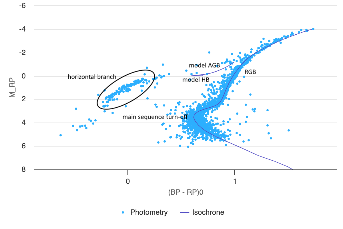
Do not try to fit the horizontal branch. As you can see in Figure 5 below, the horizontal branch in a globular cluster may appear as a prominent, spread-out population of moderately bright, blue stars — well separated from the red giant branch and sitting far to the left on the diagram. The isochrone model’s predicted horizontal branch (labelled “model HB” in the figure) does not match the data well, and the same is true of the asymptotic giant branch prediction. This is not a failure of your fit — it reflects a genuine limitation of the models. The horizontal branch involves a phase of stellar evolution characterised by pulsational instability, in which stars vary in brightness and colour by up to several magnitudes on timescales of less than a day. A static isochrone model cannot capture this behaviour. Focus your fit on the red giant branch and the turnoff point, and treat the horizontal branch as a feature to identify and understand rather than to fit.
Expect messier field star removal. Gaia’s proper motion measurements are less precise for the dense, distant stellar populations in globular clusters — especially for faint stars near the cluster core. You will need to apply relatively aggressive distance cuts to obtain a clean sample, which means accepting that some genuine cluster stars will be excluded. Unlike with open clusters, you should not expect to see a smooth, continuous distribution of field star proper motions after removal. A residual concentration near the cluster’s proper motion in the scatter plot is normal and expected.