- Open Clustermancer and use the Look Up a Cluster dialog to search for M67. Reduce the radius to 0.5 degrees, Test Radius, and click Next, then Next again to load the cluster into the Field Star Removal tool.
- Note that there are two populations of stars displayed in the proper motion scatter plot! The denser and more numerous population, centered at (pmRA, pmDE) ~ (-11, -3.5) mas/yr is M67, while the less dense population of field star proper motions is centered around (pmRA, pmDE) ~ (-1.5, -2.5) mas/yr. You can easily verify this by adjusting your Cluster proper motion limits and comparing with the color-magnitude diagram in the bottom-left: the stars at (pmRA, pmDE) ~ (-11, -3.5) mas/yr have a well-defined main sequence and red giant branch, whereas the other population is a cloud of stars indicating a wide range of distances. Can you think of a simple explanation for why the two populations would have such different average proper motions?
- Isolate the cluster’s proper motion and distance ranges as you’ve done in examples 1.1-1.4 above, leaving some extra space as you still need to fetch the rest of the archival data and can then refine limits. Don’t worry that there are some stars to the upper-left of the turnoff point in the color-magnitude diagram.
- Move to Archive Fetching, click Add Catalog Stars, and again select only the Gaia catalogue. Test Radius, and if it fails return to tighten up your proper motion and distance limits. If the catalogue data successfully load, return to refine field star removal. When you are satisfied, proceed to Isochrone Matching.
- Create the Gaia HR diagram: RP vs BP-RP. Ensure you have the Max Error value set to at least 0.15 so the three stars at the bottom-left are displayed. These are white dwarfs, the dead carbon/oxygen cores of low-mass stars that have exhausted their core hydrogen and helium fuel and previously shed off their outer layers as planetary nebulae. It is important to note that while these are in fact cluster members, you should not attempt to fit the isochrone model to these stars.
- Adjust distance (FSR mean is given, but you may also want to check the distribution on the FSR page), age, metallicity, and E(B-V) to find the set of parameters in which the isochrone model passes through the denser, single star main sequence population, up through the turnoff point and along the giant branch, and has a compact horizontal branch population at the bottom of the asymptotic giant branch. Your graph should look similar to the one in Figure 4 (though without the annotation). Download your own PNG image of this HR daigram.
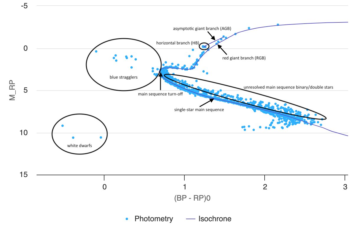
Figure 4: annotated Gaia HR diagram of M67. - Proceed to the Results Summary page where you will find estimates of the cluster’s number of stars, mass, radius, velocity dispersion, central location, as well as the parameters you entered, as well as tables of individual star data that you can download. Click Download Sources to download a csv containing astrometry and photometry data for all the stars in this cluster. Click the CSV button at the bottom-left and save a copy of the parameter values you just derived through your analysis.
- Now, open Afterglow Access in a separate window and close any open images in your Workbench. You may discard changes. Open the four BVRI images of NGC 2682 (M67) located in the “Sample > MWU > Module 5 – HR Diagrams > NGC2682” directory. With the E(B-V) value you estimated, you can now create a tri-color de-reddened image of this cluster:
- Group the BVR images and color each one appropriately, by right-clicking each image file.
- Click Color Composite Tools > Link All Layers (Pixel Value), then Color Composite Tools > Photometric Calibration, and click Measure zero points with field calibration.
- Enter the E(B-V) value you determined through isochrone matching, then click Calibrate Colors.
- Change the stretch mode to Midtone, click Default Preset, then tweak levels to your preference.
- At the bottom-right of the image click Export Image as JPG to download your dereddened color image.
- Comparing your color image to your Gaia HR diagram, you should clearly see the bright blue stars in the image that were plotted above the cluster’s turn-off point. In fact, with the data file you saved in step 6, you could identify these stars in your data set and locate them on the color image by cross-referencing their RA and Dec values. These stars are known as blue stragglers because they are massive blue stars that appear to have not evolved off the main sequence when the turn-off point reached them, so they are “straggling” behind. In general, it is important to ignore blue stragglers when fitting isochrone models because they are a result of evolutionary changes in binary star systems and are not accounted for by the models. However, their differences make them interesting stars to study!
Note: There is an important difference between the most massive young blue stars in star forming regions like IC 2948 and the stars that are designated as blue stragglers. The former may be isolated main sequence stars that simply formed later than the rest of the cluster. On the other hand, blue stragglers are thought to have formed from later stage mass transfer in binary star systems or stellar collisions, resulting in a more massive star that still has hydrogen fuel in its core, even though a star with the same mass that formed at the time that the rest of the cluster did would have already used up all its core hydrogen and evolved off the main sequence. - Note that so far, we’ve identified the unresolved binaries that lie above the single star main sequence, white dwarfs, and now blue stragglers as stars that should be avoided when matching isochrones to cluster HR diagrams.

